Task

In this project, we aim to build a JEPA-based model to predict the movement of an object in an environment that contains walls and doors. The model needs to learn and reason about the object’s trajectory, as the object can only pass through doors and will be blocked by walls.

Why JEPA

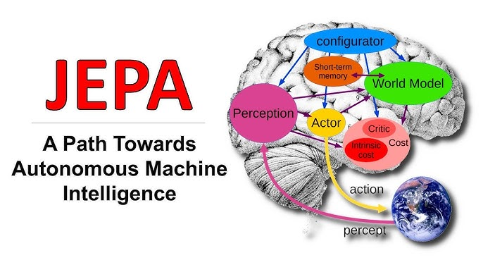
Joint Embedding Predictive Architecture (JEPA) is a self-supervised learning approach proposed by Yann LeCun in 2022. In his paper A Path Towards Autonomous Machine Intelligence, LeCun suggests that JEPA can facilitate a model’s ability to reason and plan.

We chose JEPA for this project because — aside from the fact that it is required — during inference, the only available information is the initial state and a series of actions. Thus, the model must have strong planning capabilities to predict future states based solely on this limited input, which JEPA is particularly well-suited to handle.

Data and Data Augmentation

The training dataset contains 2.5 million data points, and each sample is divided into two parts:

• Observation Tensor: Shape [B, T, 2, 65, 65].
  This means there are B trajectories, each trajectory has T time steps, and for each step, there are two 65×65 images representing the object and the environment.
  • Channel 0: Object image ([1, 65, 65])
  • Channel 1: Environment image ([1, 65, 65])
• Action Tensor: Shape [T - 1, 2].
  After the initial state, each following step is associated with an action represented by a 2-dimensional vector.

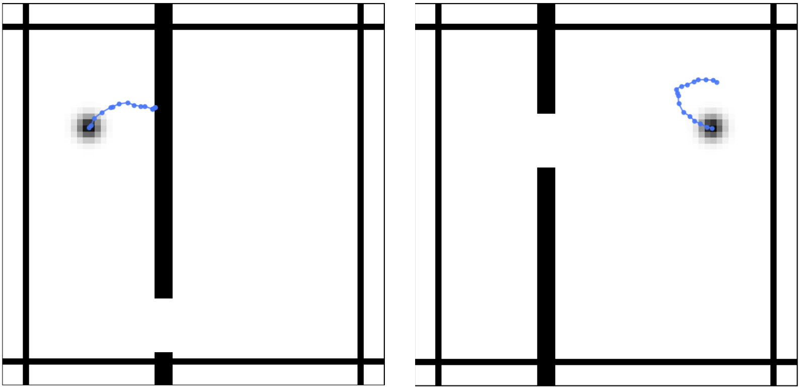Training sample

Although data augmentation is allowed, we chose not to apply it.

For this particular task, we believe that data augmentation would either have no benefit or could even degrade model performance. Here’s a discussion of some commonly considered techniques:

• Random Crop:
  We believe random cropping would be harmful for two reasons:
  • Given the sparsity of the training images, random cropping could frequently produce empty canvases, heavily skewing the training distribution.
  • Random cropping introduces counter-intuitive supervision. Suppose you crop the initial state and obtain an empty image, but the ground truth for the next step involves walls and an object. Then the model would incorrectly learn that an action can spontaneously generate structures from nothing, which violates physical intuition.

• Random Rotation or Translation:
  These could also harm model learning, for a similar reason.
  Suppose you rotate or translate an image, but keep the original action vector unchanged. In this case, the same action would lead to different visual outcomes under different spatial frames, confusing the model and disrupting the learning of consistent motion dynamics.

• Color Jitter:
  Color jitter would neither hurt nor help significantly.
  Since the images are grayscale, changing brightness or contrast would have minimal impact, and there is little color information for the model to learn from anyway.

• Noise:
  Adding noise is a tricky choice. If the injected noise is very small — so that the object’s and walls’ visual integrity remains intact — it could potentially help regularize the model.
  However, if the noise is strong enough to produce many random grey points, it would confuse the model, possibly leading it to make predictions based on noise artifacts rather than the actual object or environment layout. Or, the model cannot distinguish between noise and object, then it just make prediciton based on the wall and door instead of the object itself.

• Gaussian Blur:
  Similar to color jitter, Gaussian blur is unlikely to cause harm, but it also probably offers little benefit given the simplicity and sparsity of the task.

Model Structure

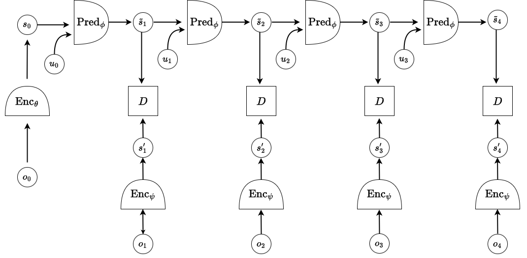
The JEPA architecture used in this task follows an autoregressive prediction framework, as shown in the diagram below.

JEPA Architecture It involves three neural network components:

• A predictor network Pred_ϕ
• Two encoders: Enc_θ for the initial state, and Enc_ψ for target observations.

In our implementation, Enc_θ and Enc_ψ are instantiated as the same network with shared weights, for simplicity — although in general, they can be distinct.

The model operates as follows:

• The initial observation o₀ is passed through encoder Enc_θ to produce the initial latent state s₀.
• Then, using the action u₀ and s₀, the predictor Pred_ϕ produces the predicted next latent state s₁.
• This predicted state s₁ is then used along with action u₁ to predict s₂, and so on — in an auto-regressive manner over time.

In parallel, for each time step:

• The ground truth observation o₁, o₂, … is encoded by Enc_ψ to generate the target representations s′₁, s′₂, ….

The training objective is to minimize the distance between the predicted latent states sₜ and the encoded ground truth representations s′ₜ at each step.

This design allows the model to learn to plan forward purely based on the initial state and a sequence of actions — without relying on access to visual inputs during inference.

Encoder

The encoder in this task is aimed to extract features from the image. As a result, when design the encoder structure, we need to choose a model that can efficiently work with image. Basically, there are two options, Vision Transformer (ViT) and Convolutional Network (CNN). In our work, we choose CNN.

There are two reasons we did not use ViT.

• First, the training set only contains 2.5M data points. According to the ViT paper, they found that ViT can perform better only on large scale of data. On ImageNet which has 1.3M data, its performance is worse than CNN. It starts to outperform CNN under ImageNet-21k which has 14M data. As a result, given 2.5M training data, we don’t think ViT can perform better than CNN since CNN has better idea about inductive bias.
• Second, modern CNN is not worse than ViT even under large training size. In the paper “A ConvNet for the 2020s”, they introduce the ConvNext network which outperform ViT both on ImageNet-1k and ImageNet-22k. Our Encoder is basically based on the ConvNext.

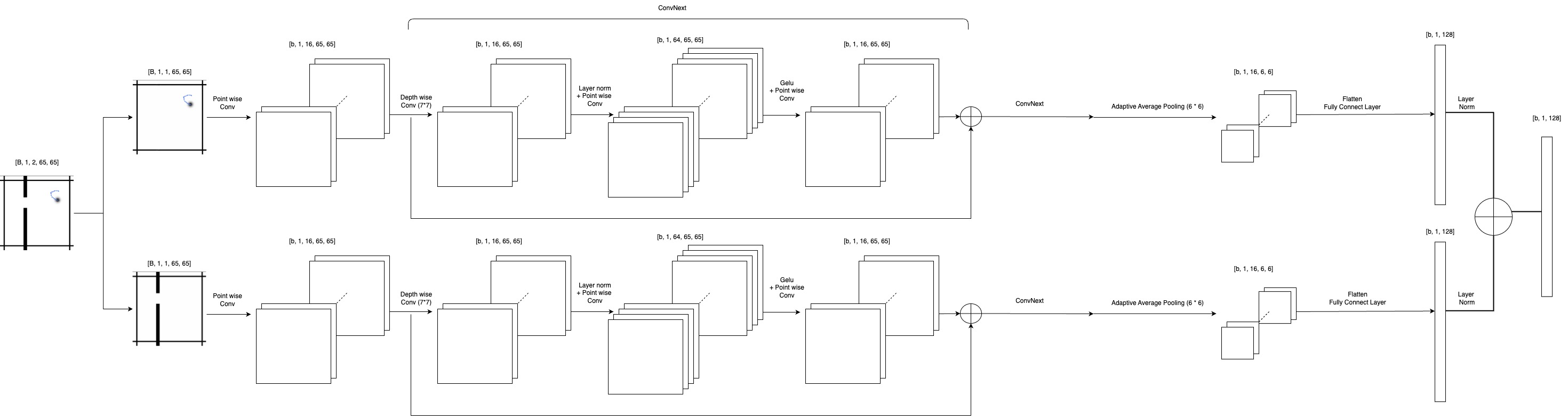Encoder

Our encoder is designed to separately process the object and environment channels, allowing the model to better capture the unique structures of each. The two channels are first split, and each passes through a point-wise convolution layer (1×1 kernel) that expands the feature dimension from 1 to 16. The expanded features are then fed through a series of ConvNeXt blocks, where each block consists of a depthwise convolution with a 7×7 kernel, followed by layer normalization, a point-wise convolution expanding the hidden dimension by a factor of 4, a GELU activation, and another point-wise convolution that projects the dimension back. Residual connections are applied within each block to facilitate information flow.

After passing through all ConvNeXt blocks, an adaptive average pooling layer reduces the spatial resolution to 6×6, and a fully connected layer further projects the flattened features into the target latent dimension. A final layer normalization is applied to each branch. The object and environment representations are then element-wise added after normalization to produce the final encoded state. The layer normalization before addition actually improves the model’s performance on distinguishing wall. Before applying layer norm, our loss for wall is 4 times higher than loss for object. With the normalization, the wall’s loss becomer smaller and is about 2 times higher comparing with object loss.

Initially, we also designed a fusion branch that jointly processed both object and environment inputs through a similar ConvNeXt structure, aiming to model cross-channel interactions more explicitly. However, due to memory limitations on a single A100 GPU, this fusion branch was removed in the final implementation.

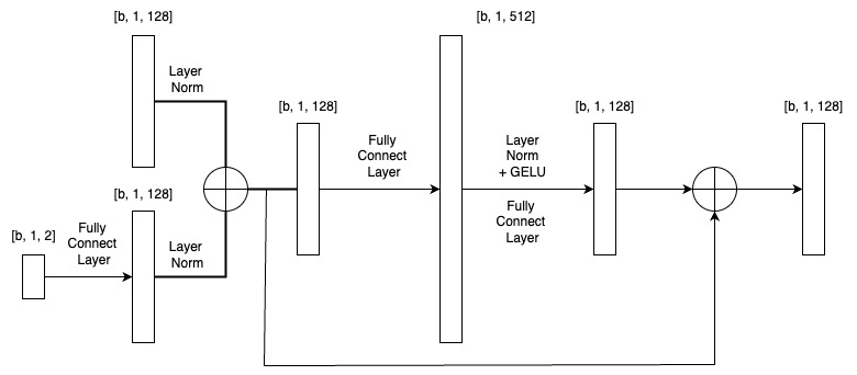
Predictor

In this model, the predictor is not responsible for extracting visual features from the input; instead, it performs affine transformations in latent space to model the dynamics between states and actions. Given its functional simplicity, we intentionally kept the predictor lightweight and designed it as a two-layer multilayer perceptron (MLP).

Predictor

The predictor takes two inputs:

• the current state representation of shape [b, 1, 128]
• and the action vector of shape [b, 1, 2].

The action is first projected to the same latent dimension (128) via a fully connected layer. To prevent either input from dominating, both the state and the action embedding are normalized independently using LayerNorm, and then added element-wise to form a joint representation. This sum is passed through a two-layer MLP:

• The first linear layer expands the feature dimension from 128 to 512, followed by LayerNorm, GELU activation, and another linear layer mapping it back to 128.
• Finally, a residual connection is applied by adding the original normalized state input to the MLP output, forming the predicted next state.

This simple yet effective design allows the predictor to model complex transitions in latent space without the overhead of convolutional operations.

Energy Function

What is Collapse and how to avoid

Collapse is a common issue encountered in JEPA models. When collapse occurs, the generated representations become useless and fail to capture any meaningful information about the input. Why does this happen in self-supervised learning models like JEPA?

The root cause lies in the lack of explicit labels: the model only attempts to align two outputs — one from the predictor and one from the encoder — without external supervision. A trivial solution the model might find is to learn invariance among training samples, where both the predictor and the encoder produce nearly constant outputs regardless of the input. From an energy-based model perspective, collapse corresponds to a poorly shaped energy surface, where low-energy points are fixed and uniform across different inputs.

There are several strategies to mitigate collapse. Some are well-understood theoretically, while others are empirically effective but less fully explained. In this blog, we focus on two major approaches: contrastive learning and regularization-based methods.

Contrastive Method

Contrastive methods address collapse by explicitly shaping the energy landscape:

• Correct pairs (i.e., matching predicted and encoded representations) are encouraged to have low energy.
• Incorrect pairs (i.e., mismatched states) are pushed to have high energy.

In our case, the idea would be to design a loss function that makes the predicted state and the corresponding encoded state as close as possible, while pushing apart predicted states and encoded states from unrelated steps.

Ideally, the energy landscape should have sharp wells at correct pairs (low energy) and high energy elsewhere.

However, in practice, contrastive methods require a large number of negative samples to adequately shape the energy surface. Since the input space is effectively infinite, it is infeasible to cover all possible incorrect pairs. Unseen negatives may still lie in low-energy regions, potentially degrading model performance.

Because of this heavy sampling requirement, we did not adopt contrastive methods for this project.

Regularization Method

Instead, we use a regularization-based strategy.

The intuition is that collapse happens when the output space shrinks — representations gradually contract toward a few points or even a single point. To counteract this, regularization methods introduce forces that encourage diversity and prevent the collapse of the output space.

By explicitly penalizing overly simple or low-variance outputs, regularization acts as a balancing force, maintaining a rich, structured latent space even without contrastive negatives.

This approach is simpler to implement and avoids the heavy sampling burden of contrastive methods, making it more practical for our setup.

VIC Regularization

VIC regularization is an idea to combine invariance, covariance and covariance [5]. The basic idea is same as the previous section, that we want the model’s output to represent different information.

Train

Training Strategy and Resource Constraints

Due to limited computational resources—particularly GPU availability—we trained our JEPA model for 35 epochs with a batch size of 128. The model appeared to converge around the 30th epoch. From our current perspective, and when comparing against the general loss performance of other teams, we believe the model has reached a performance bottleneck largely due to insufficient generalization capacity.

Training Configuration

We adopted a stage-wise training strategy. For the invariance loss, we used Mean Squared Error (MSE) as defined in the VIC framework. Optimization was performed using Adam with weight decay, and a cosine learning rate scheduler was applied to stabilize training in the later stages.

The training was split into two phases:

• In the first 30 epochs, the primary objective was to prevent representation collapse. During this phase, the variance loss was weighted more heavily than the invariance loss.
• In the final 5 epochs, we increased the weight of the invariance term to encourage the model to focus more on improving prediction performance.

Result

The results are encouraging: my model ranked 8th out of 30 teams. In terms of training loss, its overall performance is nearly on par with the 4th to 7th ranked models, with only marginal differences.

What’s more notable is the model’s efficiency—mine contains only 290K parameters, which is 10 to 20 times fewer than those ranked above it. This demonstrates a strong trade-off between performance and model complexity, highlighting the effectiveness of lightweight design under resource constraints.

Potentail Improvement

Based on the final performance of all top 10 models, our approach performs comparably—if not slightly better—than the 4th to 7th ranked models on simple test cases. However, our model exhibits relatively high training loss and struggles with complex or extreme motion trajectories. This strongly suggests a need to enhance its generalization capability.

A straightforward way to address this is to increase model capacity, such as doubling the number of ConvNeXt layers and expanding the hidden dimension. Given our current parameter count (290K), even with such scaling, the model would likely remain the most compact among the top 10.

Another potential improvement is to decouple the decoders for moving objects and static structures (walls). In most scenarios, only the object moves while the wall remains fixed. This opens up the possibility of encoding the wall once using a dedicated wall encoder, then reusing its representation across all prediction steps. In the current design, the predictor may be unable to distinguish between object and wall features purely based on their numerical representation, which could lead to overly state-driven decisions in later stages.

Additionally, we are considering integrating a DenseNet-style architecture into the predictor. By concatenating previous outputs with the current input—possibly with decaying weights based on temporal distance—the model may better capture long-term dependencies. This would allow it to condition future predictions not only on the most recent state but on the full sequence of past predictions, potentially improving accuracy for complex trajectories.

One More Thing

During the final presentation on May 5th, I gained several valuable insights from the winning team’s approach that are worth highlighting.

The winner’s model stood out by relying heavily on deterministic feature extraction methods. Rather than learning every representation end-to-end, they used algorithmic components to encode the input more directly (but also with neural network somewhere in the encoder, otherwise it will not be a JEPA model). As a result, their model achieved the best performance among all teams with only 20K parameters—a remarkable feat. This underscores an important lesson for data scientists and machine learning engineers: sometimes, simplicity and domain knowledge can outperform complex models. When possible, incorporating deterministic logic can make models both lighter and more interpretable.

Regarding representation collapse, the presenter shared an interesting insight: removing bias terms from layers may help mitigate collapse. This makes intuitive sense—bias terms can enable the model to converge to trivial solutions by zeroing out weights and relying on constant biases. Without bias, the model is more constrained and less likely to “cheat” by collapsing to a degenerate solution.

Additionally, Yann noted that the use of softargmax (often referred to as softmax) in the winner’s architecture helped prevent collapse. By treating the prediction task as a form of classification, the model could leverage contrastive learning dynamics, which naturally promote diversity in representations and reduce the risk of collapse.

Reference

[1] LeCun, Yann. “A path towards autonomous machine intelligence version 0.9. 2, 2022-06-27.” Open Review 62.1 (2022): 1-62. OpenReview
[2] Project Requirement Repo. Github
[3] Dosovitskiy, Alexey, et al. “An image is worth 16x16 words: Transformers for image recognition at scale.” arXiv preprint arXiv:2010.11929 (2020). arXiv:2010.11929
[4] Liu, Zhuang, et al. “A convnet for the 2020s.” Proceedings of the IEEE/CVF conference on computer vision and pattern recognition. 2022. arXiv:2201.03545
[5] Bardes, Adrien, Jean Ponce, and Yann LeCun. “Vicreg: Variance-invariance-covariance regularization for self-supervised learning.” arXiv preprint arXiv:2105.04906 (2021). arXiv:2105.04906