ResNet Sparse Distillation
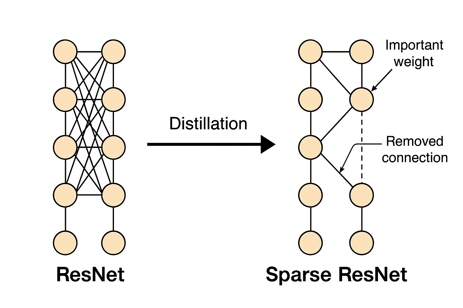
The increasing depth and width of neural networks improve accuracy but also raise hardware requirements and slow down inference. This project proposes a distillation loss function that enables immediate weight and activation pruning on the student model after distillation.
Task
In recent years, neural networks have grown deeper and wider, with more trainable parameters. This leads to higher hardware demands. On mobile and embedded devices, running fast and accurate inference with limited resources has become increasingly important. As a result, building compact and efficient models is now a key research focus.
One approach is to optimize trained models by removing operations that have little impact on performance, reducing inference cost. Pruning, both weight pruning and activation pruning, is a common method under this idea. Another approach is to design smaller models with naturally lower computation. Although smaller models often perform worse, knowledge distillation can help transfer the performance of large models to smaller ones, enabling them to achieve good accuracy with less computation.
However, pruning faces a challenge: without fine-grained retraining, the pruning results are often not optimal and fail to reach high sparsity. Knowledge distillation, while effective in reducing computation by training smaller models, does not consider sparsity. As a result, distilled models still perform poorly when directly pruned.
Contribution
In this project, we aim to train the student model to achieve both high accuracy and high sparsity. To do this, we propose a distillation loss function that includes regularization technic and sparsified teacher output distribution. With this loss, the student model can directly do zero-shot pruning both weight and activation, while still maintaining good performance.
Method
L1 Regularization
First, we focus on improving weight pruning performance. Before introducing our method, it’s important to explain the reason we think that why direct weight pruning often performs poorly. From a gradient perspective, if a certain pixel has little impact on the final prediction, its corresponding loss will be small. This results in a small gradient for the associated weight during backpropagation. Over time, these unimportant weights stop receiving enough gradient updates to decrease further. As a result, their values are just not small enough, making it hard to identify and prune them based on magnitude alone. This explains why direct pruning struggles to achieve high weight sparsity.
Regularization offers a solution. From the same gradient perspective, we can see that adding an extra gradient to the weights could help reduce them, even when the loss gradient is small. Regularization does exactly that. L1 regularization adds a constant gradient of ±1, while L2 adds a gradient proportional to the weight value. With regularization, even weights with weak loss gradients still get updated, helping push unimportant weights closer to zero and improving pruning effectiveness.
 Regularization
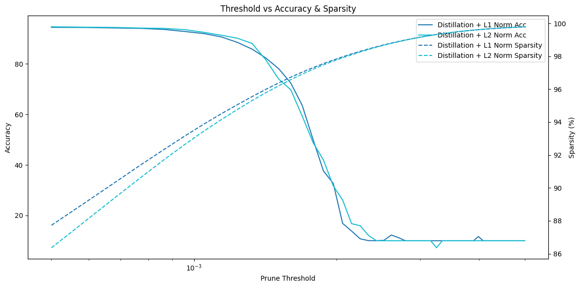
To choose the appropriate regularization method, we refer to [1], which suggests that L1 regularization works better when the model is not retrained after pruning, while L2 performs better if retraining is allowed. In our design, the student model is pruned immediately after distillation without further retraining (i.e., zero-shot pruning). Therefore, L1 regularization is a better choice.
To validate this choice, we compared L1 and L2 regularization in our experiments. We found that models distilled with L1 regularization achieved higher sparsity under the same pruning threshold, while maintaining similar accuracy to those trained with L2.
 L1 vs L2
Soft KL Divergence
Next, we focus on improving activation pruning. Ideally, the intermediate outputs of a model should be that important values should be large, and unimportant ones should be close to zero. To encourage this, we modify the teacher model’s intermediate output distribution, so the student learns from a more pruning-friendly version of it.
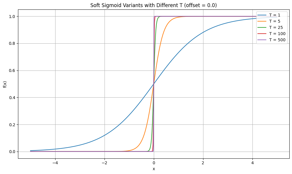
To reshape the teacher’s output distribution, we apply a soft sigmoid function. We choose sigmoid because its output ranges from 0 to 1, which makes it suitable for gating values. However, the standard sigmoid is too smooth in the middle range, meaning large values can get mapped to relatively small outputs. This weakens the preservation of important activations.
To address this, we modify the sigmoid by introducing temperature and offset. This allows us to adjust its sharpness and range, giving us precise control over how much the output is gated.
 Soft Sigmoid
The temperature parameter controls the slope of the soft sigmoid in the middle range. A higher temperature makes the curve steeper, reducing the range of values that are affected. When selecting the final temperature value, we took a very conservative approach. We chose 10,000 as the temperature, which means the function has minimal effect on outputs larger than around 0.002.
 Soft Sigmoid Temperatrue
The offset parameter provides precision control over the mapping. Our idea is, if we want to use 0.001 as the pruning threshold, slightly larger values, like those between 0.002 and 0.005, might still have little impact on the final result. If we can map these values closer to 0.001 during training, the student model can learn a more compact and focused activation distribution, which helps with activation pruning.
The offset is designed to control this mapping. For example, if we want to map 0.005 down to 0.001, then the sigmoid output for 0.005 should be around 0.2. Since we’ve already defined the soft sigmoid formula earlier, we can easily derive the offset needed to achieve this mapping.
 Soft Sigmoid Offset
It’s worth noting that, in addition to temperature, the soft sigmoid formula includes an upper bound parameter x check, which can also be adjusted. We carefully considered its impact. Our initial theory was that increasing the upper bound would first improve pruning performance, then eventually hurt it. The reasoning was that a small upper bound wouldn’t shrink important outputs, while a large upper bound might mistakenly suppress them.
However, after testing several upper bound settings, we didn’t observe a clear trend matching this theory. Overall, larger upper bounds seemed to perform slightly better, but the effect was not strongly consistent. In the final model, we chose 0.005 as the upper bound, as it showed relatively good performance among the values we tested.
 Soft Sigmoid Upper Bound
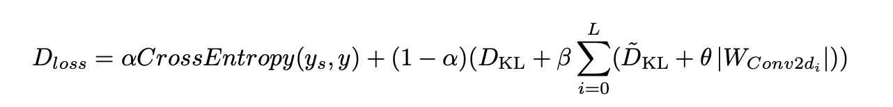
In the final soft KL divergence, we apply the soft sigmoid to adjust the teacher model’s output. The resulting function is defined as:
 Soft KL Divergence
To verify the effectiveness of the soft KL divergence design, we distilled two student models, one using standard KL divergence and the other using soft KL divergence, and compared their FLOPs under different pruning thresholds. We found that the model trained with soft KL divergence achieved slightly higher accuracy at the same threshold. Although its FLOPs were also slightly higher, the difference was small and within the same order of magnitude.
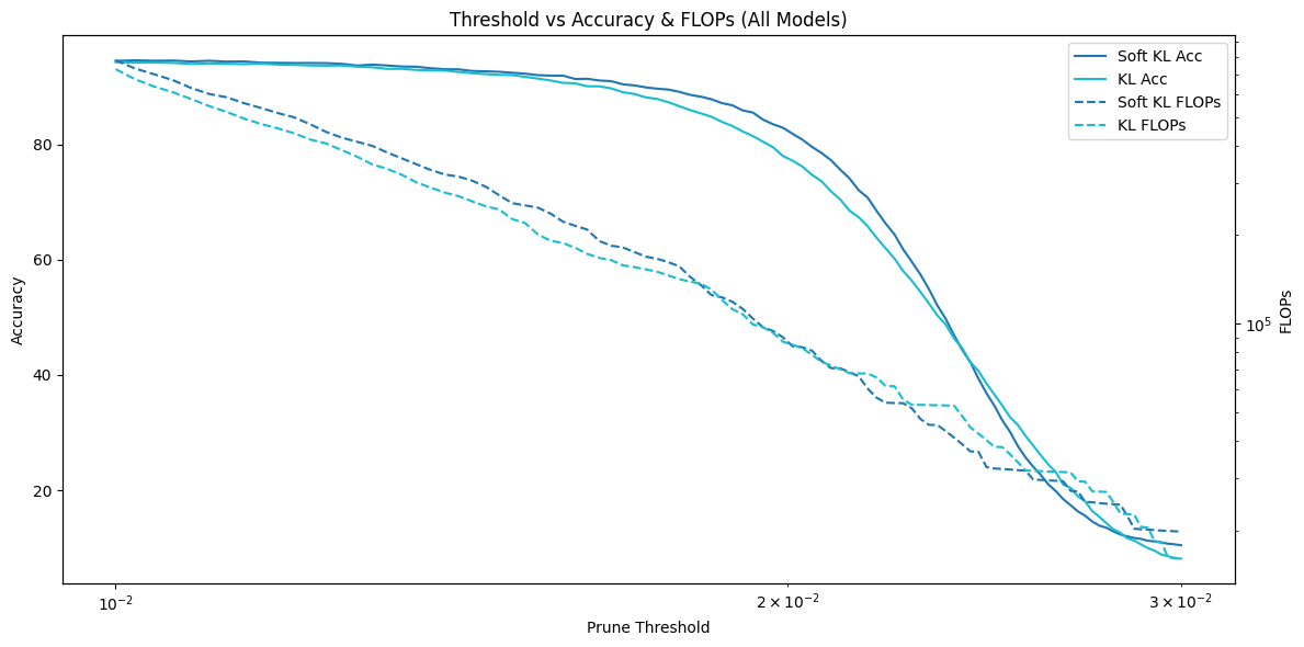 Soft KL Divergence vs. Standard KL Divergence
Distillation Loss
The final distillation loss combines the two components mentioned above. It can be expressed as:
 Distillation Loss
We set alpha = 0.1 because we want the student model to focus more on learning the sparsified outputs from the teacher and effectively control the magnitude of its weights. We set beta = 1 to give equal importance to the soft KL divergence from the intermediate layers and the KL divergence from the final output. For the regularization term, we chose theta = 1e-5, as this value worked well in our experiments.
A few important notes:
First, we applied regularization only to the convolutional layers, not to the linear layers.
Second, our soft KL divergence is applied only to the outputs of the intermediate blocks. For the final output, we still use the standard KL divergence.
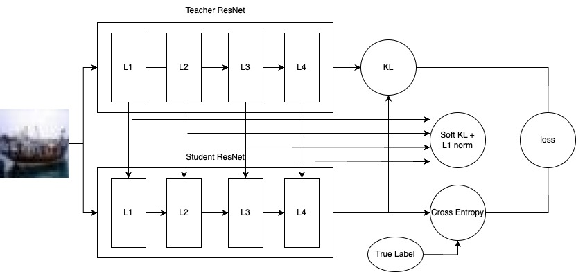 Distillation Diagram
Evaluation
We used CIFAR-10 for training and testing. Since simple ResNet models can already achieve strong performance on CIFAR-10, this allows us to focus on evaluating pruning effectiveness. The dataset is also small, which makes it easier to quickly adjust models and distillation methods.
In total, four models were evaluated:
- ResNet18 Base Model – trained directly on CIFAR-10 without any distillation or regularization.
- L2-Pruned ResNet18 – obtained by applying L2 pruning to the base model followed by retraining.
- Distilled ResNet18 – trained using our proposed distillation loss function with a ResNet18 teacher.
- Distilled ResNet18 (ResNet34 Teacher) – trained using the same distillation loss but with a ResNet34 as the teacher.
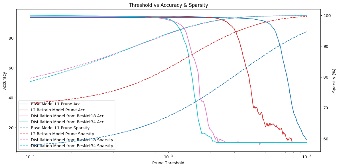
Weight Pruning
First, we evaluated the effectiveness of weight pruning. The distilled models began to show accuracy drops at smaller pruning thresholds, indicating improved weight separability. At the same accuracy level, the distilled models achieved higher sparsity compared to the other two models.
 Weight Pruning Performance
We also compared the highest achievable weight sparsity when the accuracy drops by 1% and 5%. On average, the distilled models achieved 2–3% higher sparsity in both cases.
| Sparsity 1% Acc Drop | Sparsity 5% Acc Drop | |
|---|---|---|
| ResNet18_b | 84.55% | 88.42% |
| ResNet18_b_l2 | 90.80% | 93.67% |
| ResNet18_d_18 | 92.40% | 95.16% |
| ResNet18_d_34 | 92.26% | 94.92% |
Activation Pruning
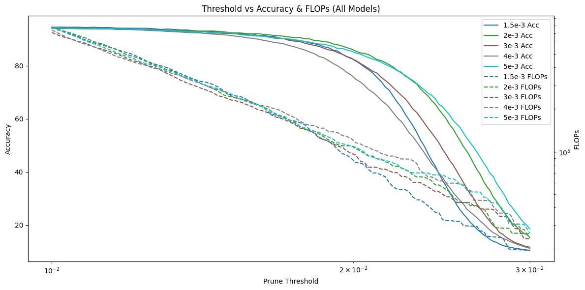
For activation pruning, we used a similar evaluation approach. Since activation pruning results can vary each time, we measured FLOPs instead of sparsity. The results show that the distilled models performed very well—at the same accuracy level, their FLOPs were up to one order of magnitude lower than the other two models.
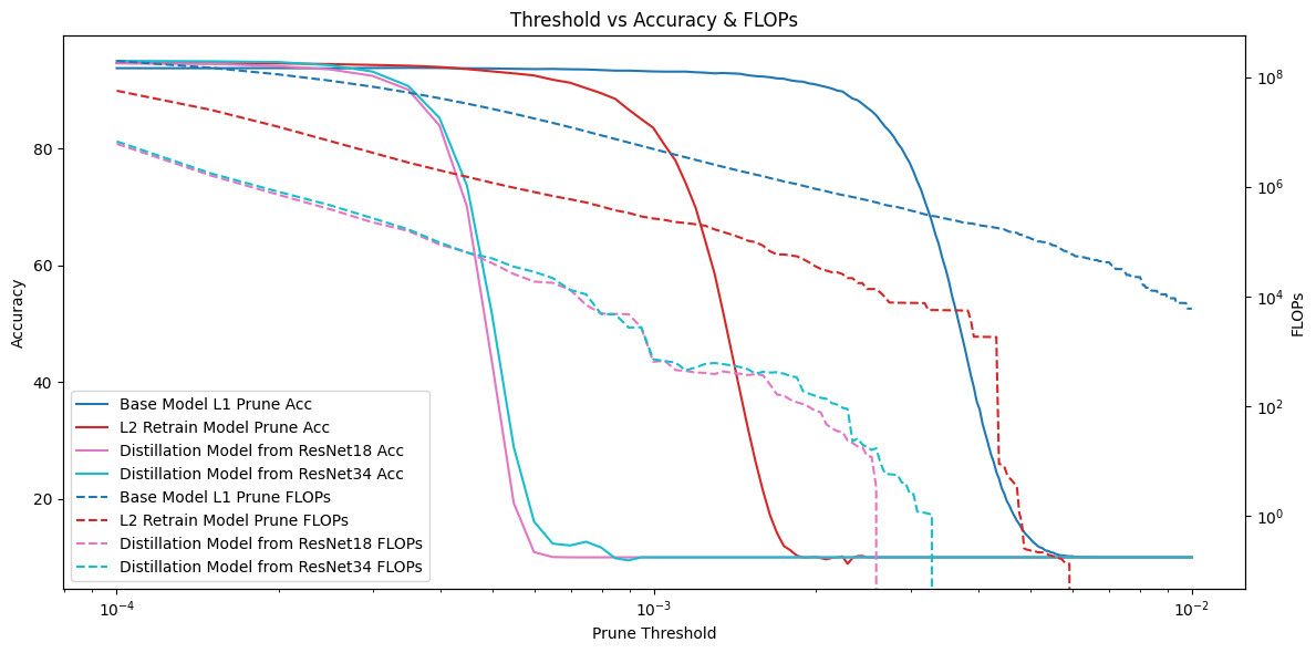 Activation Pruning Performance
Additionally, in the 1% and 5% accuracy drop scenarios, the FLOPs of the distilled models were reduced by 4 to 5 times.
| FLOPs 1% Acc Drop | FLOPs 5% Acc Drop | |
|---|---|---|
| ResNet18_b | 2,145,699 | 652,083 |
| ResNet18_b_l2 | 1,515,353 | 436,349 |
| ResNet18_d_18 | 392,288 | 145,507 |
| ResNet18_d_34 | 345,217 | 141,789 |
Discussion
Evaluating joint pruning requires testing activation pruning performance under various weight pruning thresholds, which demands significant computational resources and time. Due to resource constraints, we did not conduct joint pruning experiments.
Additionally, our distillation loss may not perform as well on Transformer-based models. Prior to this work, I attempted to prune patches in a ViT model using direct regularization, but the model failed to converge. This suggests that applying our distillation loss to ViT may also lead to suboptimal results.
Reference
[1] Song Han, Jeff Pool, John Tran, and William J. Dally. Learning both weights and connections for efficient neural networks, 2015. arXiv:1506.02626
JEPA Architecture Probing Model